Linear Algebra, Part 3: Linear Combinations and Matrix Notation

posted March 12, 2013

In this post we'll look at linear combinations and how they relate to matrix notation and systems of linear equations.

Linear Combinations

In Part 1 and Part 2 we introduced vectors and dot products. We saw that we can think of the vector sum \(\uu + \vv\) as following a path along \(\uu\) and then \(\vv\) to reach the same location as the vector \(\uu + \vv\). Another way to look at \(\uu + \vv\) is as a combination of the vectors \(\uu\) and \(\vv\), with each weighted equally:

\[ \uu + \vv = (1)\uu + (1)\vv \]

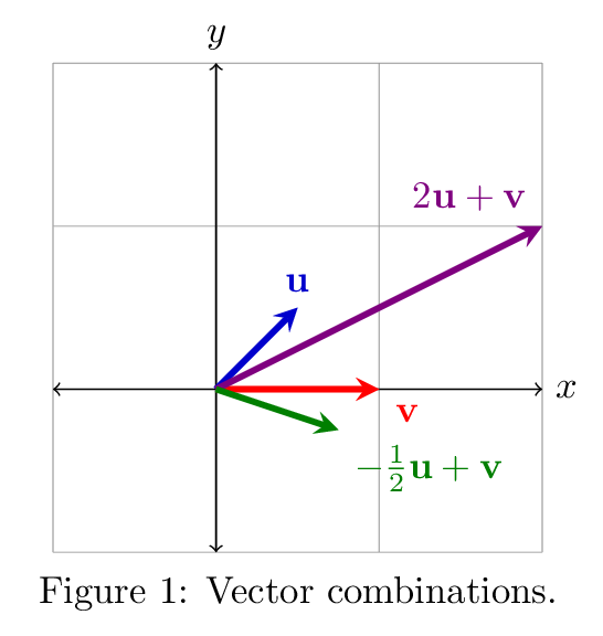
We could choose to combine them with each vector weighted differently to reach different destination vectors, as in \(2\uu + \vv\) and \(-\frac{1}{2}\uu + \vv\) (see Figure 1). Any such combination of the vectors \(\uu\) and \(\vv\) is called a linear combination of \(\uu\) and \(\vv\). A linear combination of values \(x_i\) (in this case, vectors) with coefficients \(a_i\) has the general form

\[ a_1x_1 + a_2x_2 + \cdots + a_nx_n. \]

We can think of this as combining the values \(x_i\) using the coefficients \(a_i\) to choose how much of each component will make it into the result.

Here are some examples of linear combinations:

\[ \begin{array}{ll} \text{Dot Product} & \dotp{\uu}{\vv} = \uu_1\vv_1 + \uu_2\vv_2 + \cdots + \uu_n\vv_n \\ \text{Linear equation} & 2x + y - z = 4 \end{array} \]

Linear combinations are more interesting when we combine whole vectors. For example, consider the following linear combination:

\[ 2\vxy{3}{4} + 8\vxy{1}{7} - 3\vxy{3}{0} = \vxy{5}{56} \]

The resulting vector is a combination of the vectors \(\sm{3\\4}\), \(\sm{1\\7}\), and \(\sm{3\\0}\). The combination weights each vector by a scalar amount; in this case the scalars are \(2\), \(8\), and \(-3\), respectively.

The above example can be rewritten as a pair of dot products, with the rows from the combined vectors forming dot products with the vector \(\rxyz{2}{8}{-3}\), as in

\[ \dotp{\rxyz{3}{1}{3}}{\rxyz{2}{8}{-3}} = 5 \\ \dotp{\rxyz{4}{7}{0}}{\rxyz{2}{8}{-3}} = 56 \]

We might as well factor out the right hand side of the dot products since they are the same for each "row" vector. So we rewrite this as:

\[ \begin{bmatrix} 3 & 1 & 3 \\ 4 & 7 & 0 \end{bmatrix} \vxyz{2}{8}{-3} = \vxy{5}{56} \]

We have written the original vectors in matrix notation and the left hand side of the above equation represents a matrix multiplied times a vector. This is just shorthand for the expanded dot product version we saw above. The way to read this is, "combine the vectors by taking \(2\) times the first plus \(8\) times the second plus \(-3\) times the third."

Systems of Linear Equations

So far we have been dealing only with vectors, but linear algebra is all about linear equations: equations which describe linear structures in any number of dimensions. An equation with two unknowns like

\[ x + 2y = 3 \]

describes a line in two dimensions. (You may know it better in the form \(y = mx + b\), i.e., \(y = -\frac{1}{2}x + \frac{3}{2}\), where \(m\) typically represents the slope of the line and \(b\) represents the \(y\)-intercept.) The concept extends to an arbitrary number of dimensions; here are some examples:

\[ \begin{array}{|rcl|c|c|} \hline \\ \text{Equation} & & & \text{Structure} & \text{Dimensions} \\\hline ax & = & b & \text{point} & 1 \\ ax + by & = & c & \text{line} & 2 \\ ax + by + cz & = & d & \text{2-d plane} & 3 \\ ax + by + cz + dt & = & e & \text{hyperplane} & 4 \\ & \vdots & & \vdots & \vdots \\ \hline \end{array} \]

The central motivating problem of linear algebra is to find a solution to a system of linear equations. A system of equations is a set of equations about a set of common unknowns. If we tried to put together a sensible system of equations relating the popularity of a movie over time with the price of potatoes, we would probably have trouble. But if we tried to construct a system of equations relating the position of two moving trains over time, that might make more sense.

The following is not a system of equations since it does not use the same unknowns in each equation:

\[ \begin{align*} 2x + y &= 4 \\ t + z &= 0 \end{align*} \]

However, the following example is a valid system of equations:

\[ \begin{align*} x + 2y &= 3 \\ -x + y &= 0 \end{align*} \]

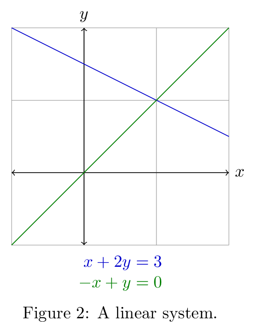
For such a system, the question that linear algebra allows us to answer is: "Is there a solution to the system?" That is, are there values of the unknowns which simultaneously solve all equations in the system? (See Figure 2.)

If we think of this geometrically, the equations above represent lines in two dimensions. If there is a solution to the system, then there are values \(x\) and \(y\) which solve both equations simultaneously. But if such values exist, that means that if we were to draw the lines, they would intersect, since for both lines the same \(x\) yields the same \(y\). This is the requirement of a system solution: that the lines, planes, etc., intersect at a single point. The system can't intersect at more than one point unless all of the equations in the system represent the same line, in which case that is not a very useful result. The other possibility is that they do not intersect at all.

When we are dealing with systems of equations, instead of writing them as we did above (with all of the uknowns mentioned in each term) we factor those unknowns out and write the system as a product of the coefficient matrix and the vector of unknowns. The following three forms are equivalent:

\[ \begin{array}{lcccr} \begin{bmatrix} 1 & 2 \\ -1 & 1 \end{bmatrix} \vxy{x}{y} = \vxy{3}{0} ~~ & \to & ~~ \begin{array}{r} \dotp{\rxy{1}{2}}{\rxy{x}{y}} = 3 \\ \dotp{\rxy{-1}{1}}{\rxy{x}{y}} = 0 \end{array} ~~ & \to & ~~ \begin{align*} x + 2y &= 3 \\ -x + y &= 0 \end{align*} \end{array} \]

Now we can look at the first form in two ways: as a series of dot products with the vector of unknowns, or as a combination of the coefficient matrix column vectors, i.e.,

\[ x\vxy{1}{-1} + y\vxy{2}{1} = \vxy{3}{0}. \]

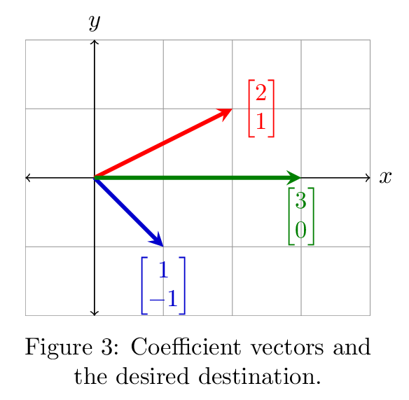
The question posed here is: is there some combination of the vectors which yields \(\sm{3\\0}\)? Figure 3 shows the answer: there is such a combination, obtained by taking one of each, so the solution to the system is \(\sm{1\\1}\). Then we have

\[ \begin{bmatrix} 1 & 2 \\ -1 & 1 \end{bmatrix} \vxy{1}{1} = \vxy{3}{0} \]

which checks out: the first vector plus the second equals the third. The solution vector tells us how to combine the coefficient vectors and it also tells us the location of the point \((x,y)\) at which the lines meet.

Afterword

Now we've looked at the idea of linear combinations, how systems of equations can be represented in matrix form, and how matrix form has a number of interpretations (dot products, combination of column vectors, and lines). Next time we'll look at elimination, the process of determining whether there is a solution to a linear system and, if so, what it is.